The chart macro in the Excel model - how to use the
chart efficiently
In the Excel model, you can easily display the figures
in the table graphically with a ready-made chart macro.
In the chart, figures are readily interpretable, and it
may be easier to change the figures, as you can see how
your estimate relate graphically to historical quarter
figures.
Though, the chart macro is easy to use and you probably
need only information how to get started i.e. where to
find that macro (1 Running the macro), here are also some
other instructions and some hints on how to deal with
the graphs.
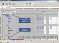
1. Running the chart macro
|
Go to the I-divQ sheet and select the Create division
chart at the macro menu and click on Run macro button.
|
Picture 1 - Click picture for full-size.
|
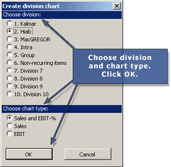
2. Choosing division and chart type
|
Choose a division you want make the chart of and
the chart type. Click then OK.
|
Picture 2 - Click picture for full-size.
|
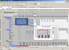
3. Moving the chart
|
A chart of the selected division and type is opened.
You can move the chart, and the possible toolbar,
by dragging them with your mouse.
|
Picture 3 - Click picture for full-size.
|
4. Excluding and including years in the chart
|
If you want to exclude one or more years from the
chart, just click on the minus sign on top of the
corresponding year. Including of a year is done
similarly, this time just click on the plus sign
of the corresponding year.
|

Picture 4 - Click picture for full-size.
|
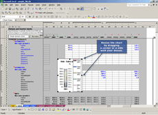
5. Resizing the chart
|
Especially, when excluding a year from the chart,
the chart may become too small to be clear anymore.
To fix this, just resize the chart by dragging one
of the corners or sides with mouse.
|
Picture 5 - Click picture for full-size.
|
6. Seeing the figure changes in the chart
|
Try the chart now and change one of the changeable
figures in the table. Remember to change the figures
of the division that is in the chart! If the chart
is on top of the division's figures, move it somewhere
else (see the point 3). Also, notice that the chart
is not updated before you verify the change in a
cell by pressing the Enter on the keyboard or selecting
another cell.
|

Picture 6 - Click picture for full-size.
|
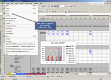
7. Saving the chart
|
To save the chart, you do not have to do anything
extra; the chart is saved as you save the excel
model, and is usable when you open the file next
time. Of course it isa also very easy to create
the charts again so you can also remove the charts.
|
Picture 7 - Click picture for full-size.
|
8. Removing the chart
|
You can also remove the chart. Remove the chart
by choosing the chart and pressing the Delete button
on the keyboard. You can easily create a chart again
by following these instructions.
|
|
|


